Material Property
|
Material properties are volume conditions in the Heat module pertaining to selected Volumes. Specify the material properties (Conductivity or Enthalpy Model), as follows: |
Conductivity
The thermal conductivity model must be defined, when Heat Module is active.
The models in the Conductivity drop down list are:
- Constant Prandtl Number
- Constant Conductivity
- Polynomial Function of T
- Cartesian Conductivity (X, Y, Z)
- Orthotropic Conductivity
- Cylindrical Conductivity
- K Matrix
Constant Prandtl NumberThe Prandtl number is a dimensionless number defined as the ratio of momentum diffusivity to thermal diffusivity. The thermal conductivity (
Here, |
||
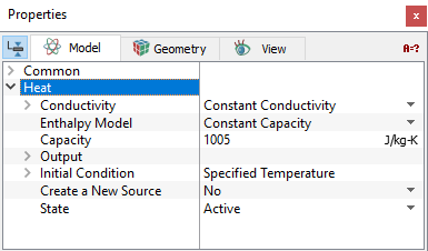
Constant ConductivityThe Constant Conductivity ( |
||
 ) for a selected volume can be specified with constant Prandtl Number (
 ) given under Prandtl Number as shown in
 and
and  is the dynamic viscosity and specific heat capacity of the fluid flow, respectively.
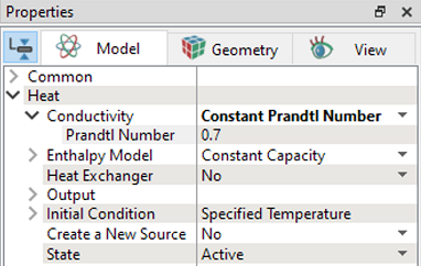
 ) is specified for a selected volume under Conductivity.
Polynomial Function of T
|
Conductivity is modelled as a function of temperature by selecting Polynomial Function of T model for a selected volume. In Simerics-MP, conductivity is specified as a function of temperature with polynomial functions using three coefficients. |
Figure 5.123 - Polynomial Function of T model |

Polynomial equation for heat capacity as a function of temperature is expressed as:

|
 = Temperature (
 )
)
 = Reference Temperature (
 )
)
 = Conductivity at Reference T (
 )
)
 = Linear Temperature Coefficient (
 )
)
 = Quadratic Temperature Coefficient (
 )
)
 = Cubic Temperature Coefficient (
 )
)
User needs to provide following parameters in the Polynomial function of T model:
- Reference Temperature: This is the temperature at which reference conductivity is calculated.
- Conductivity at Reference T: It is the constant value (
 ) in the polynomial function of conductivity.
 - Linear Temperature Coefficient: This is the coefficient of linear term (
 ) in the polynomial function of conductivity.
 - Quadratic Temperature Coefficient: This is the coefficient of quadratic term (
 ) in the polynomial function of conductivity.
 - Cubic Temperature Coefficient: This is the coefficient of cubic term (
 ) in the polynomial function of conductivity.
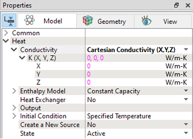
Cartesian Conductivity (X, Y, Z)
|
The Cartesian Conductivity option in Simerics-MP solves the conduction equation in solids with the anisotropic thermal conductivity specified in cartesian coordinate. Different components of thermal conductivity are entered for a selected volume under K(X, Y, Z) as shown in Figure 5.124. |
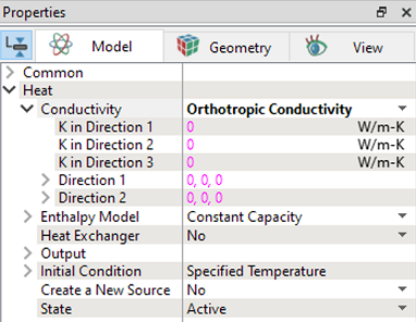
Orthotropic Conductivity
|
In Simerics-MP, an orthotropic thermal conductivity in solids is defined under Orthotropic Conductivity for selected volume. When the orthotropic thermal conductivity is used, the thermal conductivities (
|
 ,
, ,
, ) in the principal directions (
 ,
, ,
, ) are specified. The conductivity matrix is then computed as,
Since the directions ( ,
, ,
, ) are mutually orthogonal, only the first two need to be specified for three-dimensional problem. The constant thermal conductivities need to be specified for all three directions.
Cylindrical Conductivity
|
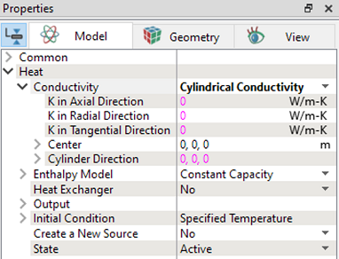
The thermal conductivity of solids can be specified in cylindrical coordinates. To define the thermal conductivity in cylindrical coordinates, select Cylindrical Conductivity in the drop-down list for Conductivity in Heat module. As shown in Figure 5.126, the center and the direction of the cylindrical coordinate system must be specified along with the radial, tangential, and axial direction conductivities. |
K Matrix
|
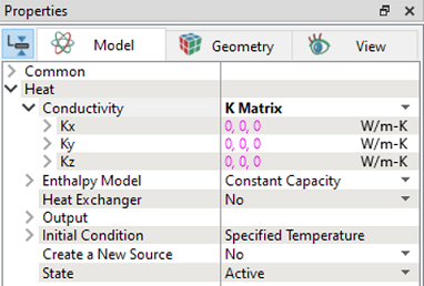
For anisotropic diffusion, the thermal conductivity matrix can be directly specified. Matrix components of the thermal conductivity as shown in Figure 5.127 can be specified in Simerics-MP. |
| Note: For information on how to perform tensor transformations of the thermal conductivity, refer 2022 ASME conference proceedings . |
Enthalpy Model
This specifies a model for computing the relationship between temperature and enthalpy.
The models in the Enthalpy Model drop down list are:
- Constant Capacity
- Polynomial Function of T
- JANAF Table
- Phase Change
- Cylindrical Conductivity
- User Defined Enthalpy
Constant Capacity
The Constant Capacity (specific heat at constant pressure  ) is specified for a selected volume under Capacity.
Polynomial Function of T
|
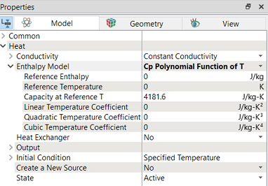
Enthalpy is modelled as a function of temperature by selecting Polynomial Function of T model for a selected volume. In Simerics-MP, enthalpy is calculated based on heat capacity of the material, which is specified as a function of temperature with polynomial functions using three coefficients. |
Figure 5.128 - Polynomial Function of T model |
Polynomial equation for heat capacity as a function of temperature is expressed as:

|
Polynomial equation for enthalpy as a function of temperature is expressed as:

|
where,
 = Temperature (
 )
)
 = Constant Pressure Heat Capacity (
 )
)
 = Linear Temperature Coefficient (
 )
)
 = Cubic Temperature Coefficient (
 )
)
 = Specific Enthalpy (
 )
)
 = Reference Temperature (
 )
)
 = Capacity at Reference T (
 )
)
 = Quadratic Temperature Coefficient (
 )
)
 = Reference Enthalpy (
 )
)
User needs to provide following parameters in the Polynomial function of T model:
- Reference Enthalpy: It is the enthalpy at reference temperature.
- Reference Temperature: This is the temperature at which reference specific heat and enthalpy are calculated.
- Capacity at Reference T: It is the constant value (
 ) in the polynomial function of specific heat.
 - Linear Temperature Coefficient: This is the coefficient of linear term (
 ) in the polynomial function of specific heat.
 - Quadratic Temperature Coefficient: This is the coefficient of quadratic term (
 ) in the polynomial function of specific heat.
 - Cubic Temperature Coefficient: This is the coefficient of cubic term (
 ) in the polynomial function of specific heat.
JANAF Table
|
The Enthalpy Model for a selected Volume can be specified directly using the JANAF Table. The coefficients for a polynomial function of temperature are entered corresponding to values from JANAF data.
This JANAF model handles a larger temperature range up to 30000 K. The temperature dependent values of specific heat ( |
Figure 5.129 - JANAF Table |
 ), Enthalpy (
 ) and Entropy (
 ) are calculated with three polynomials using 9 coefficients.
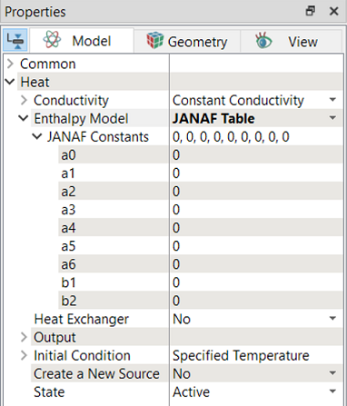

|

|

|
Phase Change
|
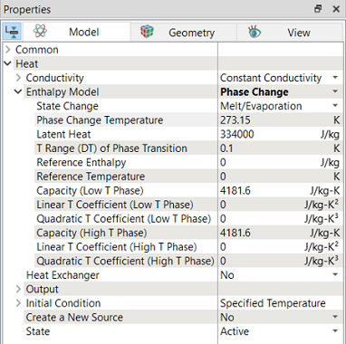
In Simerics-MP, phase change of the material is modelled using Phase Change model for selected volume. The enthalpy is calculated based on the specific heat (function of temperature) and phase of the material. The specific heat variation with temperature is provided for both phases.
|
Figure 5.130 - Phase Change model |
| Note: For information on how to model phase change, refer Windshield Defrost Tutorial. |
User Defined Enthalpy
|
The enthalpy can be specified as a function of pressure and temperature i.e., The input text file for two variables (pressure and temperature) data are created in 2-D table format and accessed using expression editor. For single variable (temperature) using 1-D table. If user has |
Figure 5.131 - User defined enthalpy |
 using the
  and temperature data and wants to provide using User Defined Enthalpy. First, fit a curve for
  as function of temperature and then integrate the curve to get the enthalpy.
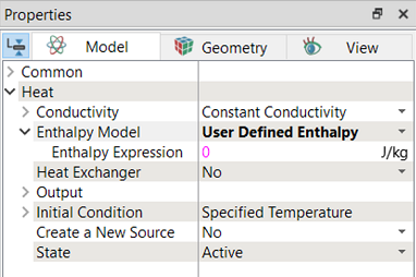
Example
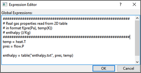
The gas enthalpy is specified as function of pressure and temperature in 2D table format, as shown in Figure 5.132. In the solver, temperature is accessed from heat module as temp=heat.T and pressure is accessed from flow module as pres = flow.P as shown in Figure 5.133. It also shows the example of how to read table from expression editor.
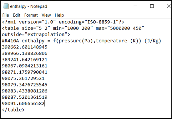
Figure 5.132 - Pressure and temperature data in 2D table format |
|
| Note: For information on how to model user defined enthalpy, refer Rolling Piston Compressor with Real Gas Tutorial. |